Quantcast
Channel: Grant Trebbin
Viewing all 99 articles
Browse latest View live

PCB Net Ties and Grounding in Kicad

$
0
0
Just a quick post this week.  I've finally gotten around to doing the PCB for my power supply and I thought I'd talk about grounding.  I'm not claiming to be an expert, I'm just trying to follow best practice and all the bits and pieces I picked up from reading textbooks and app notes.  As usual, university basically teaches you nothing about this.  You're told that the little ground symbol is zeros volts and you can dump current into it and everything will be fine, but that quickly starts to fall apart in real world situations.

Kicad power supply schematic

What you consider to be a zero impedance connection in a schematic has resistance, inductance, and capacitance.  This means that if your circuit requires large currents or high frequency to operate, that ground will no longer be zero volts.  One strategy to deal with this is to segregate grounds into different types and then combine them at a central point via a star grounding system.  This means that individual subsystems will operate with a common ground.  It also allows you to treat each ground separately.  You can use wide tracks for high current grounds, or make sure that you have tight ground loops on high frequency sections to avoid EMI problems.  Either way you need a way to deal with this when designing your PCB.

In the schematic above I've created three different grounds to help manage these issues.  An power input ground, a power output ground, and a signal ground.  The power grounds are for high current parts of the switch mode converter, and the signal ground is for the controller and low current signal conditioning circuits.  I think I have everything segmented correctly, I guess I'll find out when it comes time to test the circuit.

So you have your separate grounds, how do you connect them.  If you connect them all to a ground node, Kicad will treat them all as one net and you loose the logical separation of them.  The way to get around this is to create a component called a net-tie or pavilion ground.  It's basically a component with multiple nodes that's made of copper to connect all the nets.  It allows all the grounds to come together at one point and still keep the nets logically separated.
Net Tie
Those of you that are familiar with Kicad will know that the schematic component and footprint are separate entities, so at the moment I only have the schematic component drawn, the footprint will come later.

The Effect Of Heavy Rain On RDS Message Reception

$
0
0
In a recent post I demonstrated how to log RDS messages from FM radio stations.  As a follow up, I thought I'd share an interesting result I observed while logging data over a two week period.  I set up the equipment as described, and for most of the logging period everything worked as planned.  The receiver decoded around 13 messages per minute, sometimes more, sometimes less, but most importantly the messages were almost error free.

On the last day of logging I checked the progress and noticed that the messages contained a lot of errors, not only that, the number of messages received per minute had dropped to one or two.  I'd like to build suspense, but I knew what was wrong immediately, we were experiencing some of the heaviest rain Brisbane had seen in years.  The rain was degrading the signal from the radio station to a point that still allowed audio to be heard, but prevented decoding of RDS messages.

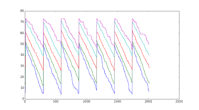
I thought it'd be cool to create a visual aid to compare historical weather data to the logged RDS messages.  Radar data from www.theweatherchaser.com was added to a graph showing how many messages were received in each 6 minute period over the two week long experiment.  6 minutes was chosen as this is the length of time between radar frames.  The frames for the animation were created using python and matplotlib.
VirtualDub was then used to convert the image sequence into a video.


I wouldn't say that there's a strong correlation between the radar images and the frequency of the received messages.  It's important to remember that the radar only shows rainfall.  There could be cloud cover or lighting strikes effecting the radio transmission that doesn't appear on the radar.  The number Hopefully it's obvious that this isn't a tightly controlled experiment, just a bit of fun. 

The file used to create the above animation can be found here.
It can't be used to recreate the animation as the source data is missing.  When learning how to use matplotlib I had trouble finding out how to do certain things.  I though placing the file here might help someone in same situation in the future.

Losslessly Compressing Similar Images

$
0
0
In a recent post, I created an animation from a series of PNG images that were programmatically generated.  Usually after a project like this I back up all the related data for archiving, but this time I wondered if I could somehow reduce the size of the images by taking advantage of temporal redundancy?  What do I mean by that?  When you look at the frames they're basically all the same and only contain slight changes between adjacent images.  Is it possible to take two images, record the difference in a way that can losslessly recreate the original image, and save space?

The method I came up is a crude simplistic implementation of how video encoding works.  Take two frames, subtract one from the other and encode the difference.  This works because the difference image usually contains very little information.  Real video encoding is much more complicated,  other frames are used to predict a particular frame, taking into account how objects in the video are moving. The prediction is subtracted from the actual frame to produce a residual image.  This is what's encoded, usually in a lossy manner.

I wanted to recreate this, but as this was a quick project, I used common file formats and software that already existed.  I didn't want to write a compression algorithm (yuck) I just needed a result.  With that in mind I decided to exclusively use the PNG file format, as it's great for compressing images with a large areas the same colour.  (I know I could use something like WEBM, MNG, or APNG, but they're poorly supported)

The plan is quite simple, take two images the same size, subtract them from each other channel by channel (including transparency) and save the difference as greyscale PNG files.  The one complication is that subtracting an 8 bit number from another 8 bit number gives you a 9 bit solution space, meaning you can't just encode the result in one image.  To get around this, the difference images are encoded as two images, the first contains the absolute value of the difference, and the second image contains the sign of the difference (negative is encoded as white).  As the image containing the sign only has two colours, one for positive/zero, one for negative, it can be efficiently encoded.

Writing a compression and decompression script in python was easy enough.  There are some peculiarities and edge cases in the PNG spec that will cause it to fail.  Everything I tested works, but I feel like there may be problems with some palette based images.

As a demonstration I processed two images that aren't similar in any way to illustrate how the system works.

PNG Images
Difference Compression Example
The two source images above are split into their RGBA channels and subtracted from each other.  You may notice that the RBG difference images have a background that isn't black, (which would imply they are equal) but dark grey, while both images have transparent sections as their background.  This is because there are in fact a different colours in the backgrounds of both images, but with the transparency set to full they look the same.  The difference image for the alpha channel also looks different, it's just black and white, this is because the images don't use graduated transparency on the alpha channel.  It's either on or off, so the difference will be either full or zero.

The 8 images on the right along with the first source image were able to reproduce the second source image.  When compared they are found to be pixel for pixel replicas apart from pixels with full alpha. The encoder I used discards the colour information of pixels that are transparent.  I'm not going to go into the file sizes and results as this was to illustrate what happens during the process.  You'd never compress these images this way.

An actual example

Below is a frame from my animation that is 1080 x 1920 pixels.  I'm going to use that as a base to compress the next frame in the animation.  I'm not going to show it, apart form the timestamp they look exactly the same to the naked eye.

Test Image
Test Frame

So, what are the results.  The image below contains the file sizes.  The original file 1.png was 347 kB.  To be fair, I ran it through PNGOUT to see how small it could be made as a standalone image.  This resulted in a 248 kB file.  In comparrison to the 8 difference and sign images, there's no contest.  In total they take up around 30 kB of space.  Around an eighth the size of the standalone image, but wait, it gets better.

List of files
File sizes


If you run the sign and difference images through PNGOUT you get a massive size reduction.

List of files
File sizes
That's right, they now come to a total of 13.3 kB, around 5.3% percent of the original file size.  The original file 1.png is able to be encoded with only 13.3 kB when using 0.png as a base image.  As a side note you probably want to throw them into a tar or zip file so the actual size on disk is reduced.
File sizes
File sizes
Although this is an interesting compression method, I would actually use it in its current form, it's a bit fragile.  I'd love to know if anyone has a similar method they use for losslessly archiving similar image. Python scripts and test images can be found on Github and Google Drive.

https://gist.github.com/GrantTrebbin/4aba7898840d96fc6b86
https://drive.google.com/file/d/0B5Hb04O3hlQSYUVzekpieEswc1U/view?usp=sharing

Simple Data Backup with Paper Based QR Codes

$
0
0
Let's say you have some important data you want to protect, how do you do it?  The obvious answer is encryption, this then leaves you with the smaller but more manageable problem of protecting the key.  This is really important though, if you loose the key, the data becomes useless.  So it's not uncommon to back it up.  How you want to safeguard the key and where you want to store it aren't the subject of this post, what I want to talk about is a method to ensure the longevity of the data and medium you store it on that's also dead easy to recover.  (It looks hard, but it really isn't)


The first thing to consider when thinking about backups is the medium.  If you archived data on a 5.25 inch floppy 20 years ago, you might have a hard time recovering that today.  First you have to find a disk drive to read the information, then you have to hope that the information stored on the magnetic media hasn't degraded, then you need to be able to read the format of the recovered file.  This doesn't just apply to magnetic media.  To quote the National Archive of Australia about the preservation of physical media:

Recordable CDs and DVDs, USB keys and various forms of flash memory have doubtful long-term reliability and are subject to format and software obsolescence.

So what do you do?  The least worst solution is to store the data on paper.  Print it out and put it somewhere safe.  If you want a bit more safety, print out multiple copies and put them in different locations, it's up to you.  If you want to get all tin foil hat, you could split the data into n pieces that only require k parts to reassemble using Shamir's Secret Sharing algorithm.  For example split the key into 6 parts that only require any 4 pieces to reassemble, then store each portion in a different location.  I'll leave that for another time.    The point is, paper has proven that it can stand the test of time if stored with even the slightest bit of care.  You also don't need need specialised equipment to read it (although it helps).

Once you decide to store the data on paper then comes the question of how you plan to do this.  If the file is binary data you can't just print it as there'll be non printable characters, and unless you choose the right font it can be hard to tell the difference between characters.  E.g. | l 1.  You could print a hex dump of the file, but if you need to recover the file re-entering that data could be a very long process.  The easiest way is to use bar codes, QR codes to be exact.  The ubiquity of QR codes leads me to believe that a major catastrophe will  have to befall humanity before we forget how to read them.  Even if it has to be done by hand, I think they're a stable format.
The process to go from file to printed QR codes and back again is surprisingly simple when you use the right tools.  There are solutions like PaperBack that accomplish a similar goal, but it seems to use it's own barcode format and doesn't use a standard like a QR code.  That brings long term reliability into question.  The method I propose is listed below and uses software with functions that can be performed manually or easily reproduced with other software.

I decided to test this out using a live USB of the TAILS operating system.  The file I've backed up is an example Keepass database I created.  Start by installing the required tools.


    sudo apt-get update
    sudo apt-get install zbar-tools imagemagick qrencode


QRencode is used to create QR codes from terminal input, and that's what we'll be using it for.
Zbar-tools is a flexible easy to use barcode reader that can decode bar codes from an image or webcam.  We're going to use it to scan the data back into the computer.
ImageMagick is like the Swiss army knife of Linux image editing.  This will be used to combine 6 barcodes onto one page ready for printing.


Create the Barcodes


Next the input file will be encoded in base 64 format.  This probably isn't needed as QR codes are capable of encoding 8-bit binary data.  I just do it to be safe.  What I did actually wastes space, so do what works best for you.


    base64 keyfile.kdb > keyfile.64


The file is then split into a series of smaller files that can be converted to QR codes.  You can only fit so much data into a QR code.  A couple thousand bytes depending on your encoding and level of error correction.  Once again, use your judgement.


    split -n 6 keyfile.64 Passwords_kdb_64


Encode each portion of the split file as a QR code.  The -l H option gives the maximum amount of error correction in case the bar code is damaged.  I've processed all files using a command line loop.  This is something to generally avoid.


    for file in ./Passwords_kdb_64*; do qrencode -l H -o $file.png < $file; done


We'll then combine 6 QR codes into one image containing 3 rows of 2 codes with the filenames under each code.  If you have more than 6 bar codes don't worry about it, imagmagick will create as many output images as you need.


    montage -label '%f' *.png -geometry '1x1<' -tile 2x3 Passwords_kdb_64.png


QR code Backup
Resulting QR codes storing a password database

Recover the Original Data


Scan each of the QR codes in order using zbarcam and redirect the output to a file.  Each code is on a new line with a header identifying the type of code scanned.  The new lines and headers need to be removed.  This was done manually.


    zbarcam > keyfile.64


The last step is to convert the base 64 encoded file back to the original binary file.


    base64 -d keyfile.64 > keyfile.kdb


There you have it, file to QR code and back again.  What I like about this method is that even if all the software used to create the final output image disappears, the encoded data can still be recovered as long as you can decode a QR code and convert a file from base64 back to binary.  Both of these processes are widely known.

You can find all the associated files below.
https://gist.github.com/GrantTrebbin/0c6aadc7ecebe3107d08
https://drive.google.com/folderview?id=0B5Hb04O3hlQSfmwzVFdCTS1YZm8xSVVLZm95by0zLVpaTHR2WE1XcTVicWE5NUFJZjg4cGs&usp=sharing


Cheap and Easy DIY TV Stand

$
0
0
Recently my mother asked me to sort out a problem she was having.  On top of a cupboard in the kitchen she has a 26 inch LCD TV she likes to watch.  It's at a height of about 2.5 meters, and when sitting, she's looking up at an angle of about 30 degrees.  At such an extreme viewing angle the image becomes unwatchable.  What she wanted was a way to tilt the TV so that the screen was facing her when she sat down.

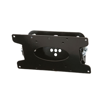
I thought this would be easy, the TV has 200mm x 100mm VESA mount points on the back, it's not too heavy (8kg), all that was needed was a stand that allowed it to be tilted down.  The cheapest bracket and stand that met our criteria was over $150 and that was more than we were willing to pay, so it wasn't going to be as easy as I thought.  I decided to just buy a tilting wall mount bracket for $35 and figure out what to do with it when it arrived.  Building my own tilt mechanism would've taken way too long and wouldn't have been as good.
Bracket
B-Tech BT7522B LCD wall mount bracket

After receiving the tilting bracket I went to the local hardware and walked around to see if I could find something to mount it to and make a TV stand.  It wasn't long until I found the post stirrup section.  Just in case you don't know, post stirrups are metal brackets used to keep timber posts of buildings elevated above ground to prevent rotting. They're concreted into the ground or bolted to a concrete base and the post is then attached to the top part.  Perfect, for $7 I get a sturdy metal bracket that can be mounted to a ply base to complete the job.

post stirrup
Post stirrup TV display stand
I just happened to have an offcut of 19mm plywood under my bed that was perfect for the base.

Plywood
Ply base
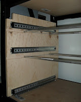
It always pays to keep large offcuts.  Originally the ply was left over from my removable drawer project.
Drawer Slide Holder
Drawer slide holder
It then became a side of my standing desk experiment.
Standing Desk
Standing desk add-on
As the stand sits on an L shaped cupboard in a corner, I had to cut out a section so there wouldn't be an overhanging bit.  To attach the post stirrup to the base board I used 4 bolts and a metal plate as a washer.  This meant that the bottom was no longer flat and needed to be elevated.  To do this I used a hole saw to cut some circular feet out of the scrap ply section that was removed.  These were glued and screwed in place.  The parts that were going to be visible when installed were then painted white.
TV Stand Base
Base with feet and washer plate attached
.
Metal Plate
Washer plate
The tilting bracket was then attached to the post stirrup with some metal screws and lock nuts.  It's not the most attractive piece of furniture, but it's not too hard to imagine how to make it look like more like a professional product.  A new piece of ply the right size and a bit more time planning, painting, and sanding, this wouldn't be out out place in a living room.  Depends how good you are at finishing wood though, I took some shortcuts because I wanted this to be a one day build.  The TV hides all of the ugly stuff anyway.  The only part you can see is the edge that I painted white

The best part however is that it only cost me $50 maybe $65 if you bought everything new.
TV bracket and post stirrup
Tilting bracket attached to post stirrup
.
TV bracket and post stirrup
Tilting bracket attached to post stirrup
.
TV Stand
Assembled TV stand
.

An Analysis of the Triple M Brisbane Playlist

$
0
0
When listening to radio in the car I do exactly what I would at home, channel surf.  Generally I listen to Triple J but also switch between Triple M, 4ZZZ, and 612 ABC for something different.  For a couple of months there was a period that every time I switched over to Triple M it seemed that they were playing The Spin Doctors.  Now any normal person would pass that off as mere coincidence and leave it there, but if you've read this blog before you're probably aware that I'm not normal.  I started to wonder exactly what type of songs were played on the station, did they play certain music at different times of the day to cater to a different demographic?  To answer this I needed to log what songs were played, unsurprisingly I chose a solution that required electronics to log the RDS messages the station broadcasts.  The method used was described in a previous post, Using a Raspberry Pi to Log Songs Played on a Radio Station.  They do list recently played songs in their on-line streaming player, but I couldn't figure out a way to easily log them.  Besides, electronics is more fun.

I've since discovered a similar analysis was done by Daniel Nitsche in 2014.

The logger was left to run for two weeks, generating a file with 273902 entries, on average logging what was being played every 4-5 seconds.  Writing software to turn that something to useful was in my opinion going to take longer to do than actually editing the file by hand as there were intelligent decision to make along the way.  There were small errors that needed correcting as well.  For example, when the daytime presenters played a snippet of the songs to be aired in the next hour, that was also broadcast on the RDS message system.  So it would appear they played the song and then played it again within the hour.  That had to be corrected.  I'm not saying this couldn't be automated, but for a one off, it's not worth it.

After editing, the data showed that there were 2805 songs played over the two week period, about 8 songs an hour.  That sounds about right.  There's probably the occasional error in my data set, but I believe it's accurate enough to show any trends.  There may also be some errors in the release year I have listed for the songs.  Initially I tried to use an on-line music database to get the release date for each song, but that was way to slow and error prone.  In the end I Googled each of the 868 songs to find out when they were released (doesn't take as long as you think, I averaged about 6 a minute).  Then comes the problem of when a song was actually released.  Some songs are released on the album but their release date is when the single comes out.  I choose when they were first publicly available.

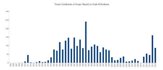
So what can we actually learn from this data?  I started with the histogram below to see the distribution of songs played.  The oldest song played was "Sympathy for the Devil" by the Rolling Stones from 1968.  Then there's a  bit of a peak in 1971 before the bulk of songs from about 1980 to 2000.  1991 seems to be a massive year for music and unsurprisingly aligns closely with the active rock format the Triple M subscribes to.  Billboard has a go at explaining 1991.  The bulk of the songs played in 1991 are from the following classic albums.

U2 - Achtung Baby
Red Hot Chili Peppers - Blood Sugar Sex Magik
R.E.M. - Out Of Time
Pearl Jam - Ten
Nirvana - Nevermind
Metallica - Metallica
Guns N' Roses - Use You Illusion I
Guns N' Roses - Use You Illusion II

The next thing to notice is that there aren't many songs from the 2000's, but they do play a lot of recent music from the last 5 years.

histogram
Yearly Distribution of Songs Played on Triple M Brisbane
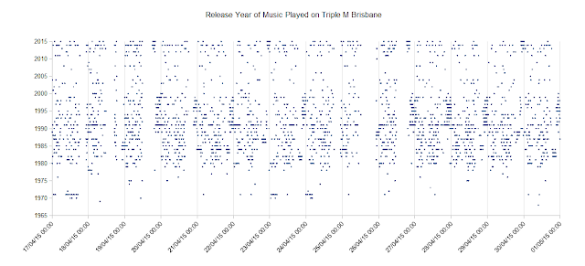
The next plot shows how the release years of songs are distributed over the two week period.  Although you can see the information from the histogram reflected here, there isn't much too much else to see here.
graph
Release Year of Music Played on Triple M Brisbane
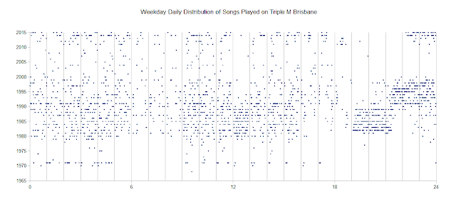
The last graph was a bit boring, but by taking the data and showing it differently we can learn some interesting things in the one below.  By plotting all the weekday data on one daily graph, patterns begin to emerge.  For instance, between the hours of 5 and 9 am it appears that there is a blackout on pre 1980 music.  You can also see that songs are less frequently played between 6 and 9 am when the breakfast crew are doing their thing.

When the drive show comes on from 4 to 6 pm you can once again see the drop off in the amount of music played to make way for the presenter.  Between 6 and 7 pm there is a sports show that plays relatively little music as well.  Then between 7 and 9:30 pm the focus seems to be on 80's music, this then changes to 90's music until about midnight.  I assume they have data that says people who like 80's music are in bed by 9:30 pm.
graph
Weekday Daily Distribution of Songs Played on Triple M Brisbane
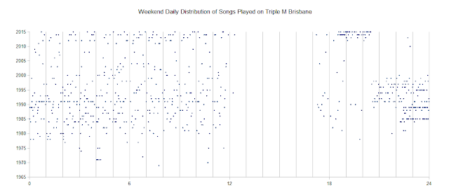
The data for the weekend shows similar patterns.  After lunch, the sports coverage starts and the music stops.  There's also a relatively dense block of new music between about 6:30 and 8:30 at night, this turns out to be a show on Sunday that plays a lot of new music.
graph
Weekend Daily Distribution of Songs Played on Triple M Brisbane
I also did up a Poincaré plot to see if any other patterns emerged, but the only thing obvious is the predominance of 1991.  If you've never seen one of these before it's a graph of data that plots data point n against (n+1).  They're very useful for finding patterns in binary files as well.
Poincaré plot
Poincaré plot - Release Year of Songs Played on Triple M Brisbane
So to wrap things up I looked at what the most popular artists were.


ArtistTimes Played
Red Hot Chili Peppers76
INXS69
Foo Fighters66
U265
Pearl Jam61
R E M56
Midnight Oil55
AC/DC44
Guns N' Roses40
Powderfinger39


I also looked at the most popular songs too.


SongArtistTimes Played
GeorgiaVance Joy26
Hold Back The RiverJames Bray19
CongregationFoo Fighters17
Blame It On MeGeorge Ezra17
Every Breaking WaveU217
CrystalsOf Monsters and Men16
Someone NewHozier15
BelieveMumford & Sons15
Two PrincesSpin Doctors 14


Ha!!!!!  Proof I'm not insane*.  Two Princes by Spin Doctors is the 9th most played song on Triple M.  Coincidentally released in 1991.

*This blog post probably doesn't help my case.  Hmmm :-/

You can find my original logs here.

https://drive.google.com/file/d/0B5Hb04O3hlQST2pKU0dHOTQ5SlE/view?usp=sharing


Large LED Panel Light Testing

$
0
0
I've recently wanted to do more videos and take better pictures for the blog, but I've been limited by my lighting.  At the moment most of my photography is done under 2 LED tube lights that illuminate the whole room.  They appear bright, but in reality there isn't enough light for photography, and although they're not as bad as point sources, I get long straight reflections on shiny objects in my photos.  What's needed is a large, bright, distributed light source that I can place above my desk.  It should remove most reflections, and also reduce shadows when working.  I've previously played around with a small LED light panel and it seemed a larger version would be perfect for the job.  After looking at all the options available on AliExpress (there are a lot),  I finally choose a single large 80W panel.

LED Light Panel
80 Watt LED Panel
This thing is massive.  It's 600mm x 1200mm x 8mm, the size of a standard ceiling tile you'd see in any Dilbert style office.  According to the specs it's an 80W panel with an output of 8000 lumens.  That gives a luminous efficacy of 100 lumens per Watt, which is a pretty standard value for white LEDs.  It has a reasonably high colour rendering index of above 80 to ensure faithful colour reproduction.  The colour temperature is somewhere around 4000K, which is the colour I'm most comfortable working under.

Electrical Specs
LED Panel Specifications
I was a little nervous ordering something so large and expensive from China.  When picking up the panel from the post office it became obvious my concerns were valid.  It was shipped in a box with the power supplies and they were allowed to freely move around.  It seems at some point a weight was placed on one end while the panel was resting on the power supplies and it was bent on the long edge by about an inch.  No problem though, I was able to easily bend it straight.

LED panel light
Meter ruler placed along the edge of the panel
.
LED panel light
Maximum deviation of the panel from straight
What's the point of buying something if I don't pull it apart?  After removing the back plate the construction method became obvious.  There are two white LED strips on the long edges of the panel, each containing around 200 x 200mW LEDs.  The panel uses the same method to get light from the edges to the face of the panel as the smaller light described in a previous post about LED panels.  There are two large thin sheets of foam to keep the plastic layers firmly pressed together with a return wire running on top of them.

LED panel light
LED panel with back removed face down
.
LED panel light
LED panel with back removed lit up
.
Pattern on back layer to disperse light
The frame is flimsy aluminium that's spot welded in the corners.  From what I can gather each part isn't overly strong but when assembled they make a fairly rigid product.  As usual in these lights, the wiring isn't great.  There isn't any significant strain relief and it looks like constant flexing of the cables could cause the solder joint to fail.
LED panel light
Welded corner and wiring
I wasn't willing to completely disassemble it as I think it'd be easy to damage if I wasn't concentrating.  I was however able to see the LED strip sandwiched in between the frame and the optical plastics.

LED Strip
LED strip
The light comes with two power supplies, which is disappointing, I would've rather paid less and bought separate power supplies as I don't intend to use these.  They're a no frills standard LED driver.  They take a multi voltage mains input and can drive an LED string at 30 to 40 Volts at 900 mA.  The astute among you may have noticed that's only a maximum of 36W.  So it's likely they're slightly underdriving the panel, which isn't a bad thing.

power supply
40W - LED driver module
I balanced the panel between the backs of two chairs to take some test shots.  I think they turned out OK.  There aren't too many severe reflections and the light seems bright and evenly distributed.  Even with the crappy point and shoot camera I use, the colours seem vibrant.

Pencil Case
Case that holds my metal files
.
Eelctroncis
Raspberry Pi
.
Electronics
DC - DC converter module
It wouldn't be right If I didn't use this panel light to pretend to be a doctor and look at some X-rays.  Luckily I had some laying around from few years ago.

X-ray
Coronal slices of my sinuses
Look at that photo.  Ain't I a handsome devil?

X-ray
The inside of my head
Overall I'm happy with the product.  Yeah, it could have been packed better but it's not a major problem and you forget about that as soon as you see it working.  It really is quite impressive to turn this thing on have it basically blind you.  The next step is to make some sort of frame to mount the light above my desk.  I think welding may have to be involved.

Raspberry Pi USB Webcam Testing

$
0
0
This post will unfortunately be very short.  I was playing around with a webcam connected to a Raspberry Pi, and just as I was starting to make headway I got sick.  I was using a Logitech C525 to take still images.

webcam
Logitech C525


I got far enough into the project to realize that the camera didn't have enough resolution for what I wanted to do.  So I need to look at other options.

Just to document what I've done I'll include the commands I was using here.  fswebcam was used to take the still images and uvcdynctrl is used to configure the camera, but it's poorly documented and I'm still trying to figure out how to use it.  You may need to install packages to use these commands.


fswebcam  -r 1920x1080 -s brightness=70% -s gain=50% -S 10 test.jpg
uvcdynctrl -L a.txt
uvcdynctrl -s "Focus (absolute)" 220


I promise I'll do better next week.

Controlling a USB Relay with a Raspberry Pi

$
0
0
I love the Raspberry Pi.  It allows me to prototype ideas quickly and without too much effort, but one thing I despise is the GPIO.  Maybe despise is too harsh, but it's a clunky way to interface electronics to what is for all intents and purposes a striped down personal computer.  Don't get me wrong, the GPIO needs to be there and I've made use of it before, but if I want to quickly prototype something I have to spend time figuring out how to use it and then I've got jumper wires all over the place.  I much prefer to use devices that are connected to the USB port.  They can be easily reused on other computers and the final solution is much neater.

Recently I've been toying around with a project that needs to switch a load on and off.  It's a low voltage LED light so nothing too complicated, and I have no problem figuring out how to switch the load via a transistor connected to one of the GPIO pins, but everything gets messy and then I have to do up a small prototype board to mount the parts on.  You know what would come in handy?  A USB controlled relay.  Unsurprisingly someone has already thought of that, they're all over eBay and Aliexpress, some are controlled as USB HID devices and some use the good ol' USB to UART method.  I bought a couple of the USB to UART style devices from www.lctech-inc.com to play around with, and at $10 AUD each it's not worth my time to come up with a custom solution.

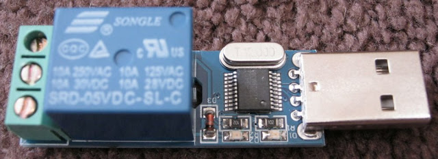
Electronics
Top Side of PCB
There's not much to the module.  As you can see above it's what you'd expect.  A USB connector, a relay, a set of terminal, and a few electronic components.  When plugged in, you send commands to it over a virtual com port to turn the relay on and off.  There are two status LEDs, one to indicate the device has power and another to indicate the relay is active.  Couldn't be easier.

Electronics
PCB Mounted Relay
The Songle relay used seems to be the de-facto standard in this area of the market.  It's a standard NC/NO relay that can be switched by applying 5 Volts to the coil.  The data sheet isn't too clear but requires 90 mA or less to actuate the relay.  The contact resistance of 100 milliOhm isn't the worst I've seen either.

Between coil & contact - 1500VAC 50/60HZ (1 minute)
Between contacts - 1000VAC 50/60HZ (1 minute)

The relay is sufficiently rated for mains voltage use and has adequate isolation, but I wouldn't use it.  I don't like running mains voltage through random crap I bought off eBay.  Besides that, even if the relay is rated for 10 Amps, I'd be surprised if the tracks on the PCB (hidden under the relay) are up to the job.  The connector definitely looks like it's not rated for that much current.  Based on that, this device will only be used for low voltage medium current applications.

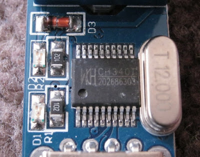
Electronics
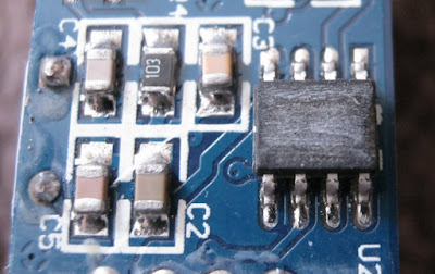
CH340T USB to Serial Controller
As mentioned before, the relay is controlled by sending commands over a USB to serial converter.  In this case a CH340T IC is used.  The only data sheet I could find for this chip was in Chinese and wasn't very helpful.  The Raspberry Pi has the drivers by default and I've read that the latest versions of Windows do as well.  Disappointingly, the serial number of the devices aren't set or are unable to be read in Linux.  This has the side effect that you can't connect two of these relays to a computer and deterministically know which relay is which.  In Linux, if two devices are plugged in at once they enumerate at /dev/ttyUSB0 and /dev/ttyUSB1, but you can't be certain that they enumerate in the same order if you reboot.  I'd hoped that I'd be able to tell them apart by reading the serial number of the USB devices, but as they aren't set, no luck.  It doesn't really matter, I only need to use one of them, but if I did need to use 2 devices I could buy a two relay board.

Edit - Bingo.  I think I've found a way to do it by using the physical mapping of the ports.

pi@raspberrypi ~ $ ls -l /dev/ttyUSB0
crw-rw---T 1 root dialout 188, 0 Jul 22 19:46 /dev/ttyUSB0


pi@raspberrypi ~ $ ls -l /sys/dev/char/188:0
lrwxrwxrwx 1 root root 0 Jul 22 20:01 /sys/dev/char/188:0 -> ../../devices/platform/bcm2708_usb/usb1/1-1/1-1.3/1-1.3.1/1-1.3.1.3/1-1.3.1.3:1.0/ttyUSB0/tty/ttyUSB0

pi@raspberrypi ~ $ lsusb -t
/:  Bus 01.Port 1: Dev 1, Class=root_hub, Driver=dwc_otg/1p, 480M
    |__ Port 1: Dev 2, If 0, Class=hub, Driver=hub/5p, 480M
        |__ Port 1: Dev 3, If 0, Class=vend., Driver=smsc95xx, 480M
        |__ Port 3: Dev 5, If 0, Class=hub, Driver=hub/4p, 480M
            |__ Port 1: Dev 7, If 0, Class=hub, Driver=hub/4p, 480M
                |__ Port 3: Dev 20, If 0, Class=vend., Driver=ch341, 12M
                |__ Port 4: Dev 10, If 0, Class=stor., Driver=usb-storage, 480M
            |__ Port 3: Dev 8, If 0, Class=vend., Driver=r8712u, 480M
        |__ Port 5: Dev 9, If 0, Class=HID, Driver=usbhid, 1.5M


The 1-1.3-1.3:1.0 string describes the physical layout of the USB device.  The device is plugged into port three of the first hub which is plugged into port three of the second hub which is plugged into the Raspberry Pi.  I've highlighted the important bits to make it a bit clearer.  BTW The reason I use two hubs is because I have a USB 3.0 hub connected to the Pi and the USB 1.0 USB to serial converter needs to be connected to a USB 2.0 hub for the pi to see it.  It's a bug with the Pi.

Electronics
Bottom Side of PCB
The quality of the board isn't too bad.  All the SMT parts that are automatically placed have nice clean solder joints, but the hand soldered through hole parts leave a lot to be desired.  There's a lot of flux residue on the board and the pads are too small causing the solder to ball up on the leads resulting in weak joints.  I have to give them points for routing out an isolation slot in the board though.

Operation is pretty self evident.  The SOT-23 transistor Q1 is used to apply current to the coil of the relay.  If you look at the top of the board there's also a reverse biased diode placed across the relay coil to stop back EMF spikes.

Electronics
IC with Markings Scratch Off
The IC on the top handles the USB to serial conversion, but the serial commands still need to be interpreted and used to control the relay.  I assume the IC on the bottom side of the board with its markings removed is some sort of micro-controller to do this.

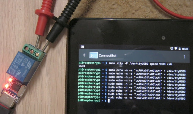
Controlling the relay is dead simple

You first need to configure the serial port at 9600 baud with a character size of 8 bits.

stty -F /dev/ttyUSB0 speed 9600 cs8

Then you send the command (in hex of course) A0 01 00 A1 to close the contacts

echo -n -e '\xA0\x01\x00\xA1'> /dev/ttyUSB0

Then you send the command A0 01 01 A2 to open the contacts.

echo -n -e '\xA0\x01\x01\xA2'> /dev/ttyUSB0

Tablet and Relay
Testing the Relay
I think these are great for prototyping.  Not only can I use this on a Raspberry Pi, I can use it on a desktop computer or possibly a phone or tablet (not tested).  It's also great for people that are coming from the software world who may not be comfortable interfacing with the GPIO port of the Pi.  They can plug it in and deal with what they know best (software), and within a few minutes control devices like fans, pumps, lights or whatever else you could imagine.

8MP Aliexpress ELP Webcam

$
0
0
I've recently been thinking about using the Raspberry Pi for image processing and wanted to use a Logitech C525 web cam that I'd bought earlier in the year.  It quickly became apparent that its resolution was less than expected and although it'd probably be fine, I didn't want the image quality to be the limiting factor of my project.  The next step was to start looking around for cheap web cams on my favourite Chinese sites.

I wanted a reasonable image quality and resolution for a decent price, and luckily enough it turns out that this isn't too hard to find.  A store on AliExpress called Ailipu Technology was selling an ELPCCTV brand 8 MP USB web cam for approximately 85 AUD.  I'll get into the specs later on, but first I want to look at the construction as it differs from a standard retail web cam.

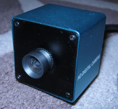
WebCam
ELP-USB8MP02G-L75
The camera is a cubic shape made of an extruded 40 mm aluminium profile with metallic front and back plates.  The camera is mounted to the front plate with a manually adjustable lens protruding out approximately 10mm.

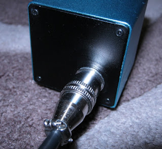
WebCam
Back of Web Cam
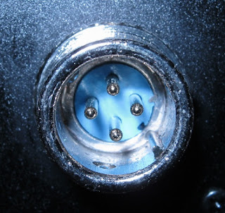
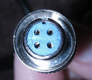
The USB cable is removable and is connected with a 4 pin locking connector on the back plate.  I assume this allows easier installation if it's used as a security camera.  Most of the products the company sell are marketed to the security industry.

Connector
Web Cam Connector
At the bottom of the connector in the image above you can just see a small metal ball that's used as part of the locking mechanism.

Connector
Web Cam Connector
The outer part of the connector in the image above is a retractable shell that locks the plug in place when it's inserted.

So now for the specs.  The camera has a claimed resolution of 3264 x 2448 and uses a Sony IMX179 sensor.  It turns out that this seems to be the same sensor used in the Nexus 5 phone from 2013.  The business model that the company appears to use is it to take old excess phone image sensors (could possibly be a lower grade) and re purpose them as web cams.  The sales page claims 15 frames per second at maximum resolution but that seems a little far fetched.  I've only been able to get 2 fps which seems more realistic for a USB limited connection.

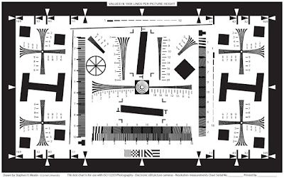
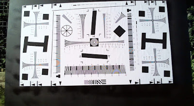
Before using the camera I wanted to be certain that the stated resolution was real and not some made up interpolated number.  In the past I've seen webcams that market themselves at the interpolated resolution which in my opinion is a blatant lie.  To do this I found an ISO12233 test chart from Cornell University and used it to verify the cameras specifications.

The process is simple, take some photos of a high quality printed version of the chart, and then analyse the image to observe the resolution limits.  I went to the local office supply store and had an A1 version of the test chart printed for a couple of dollars and then glued it to 600 x 900 mm Masonite panel that had been painted black.

Test Pattern
ISO 12233 Test Chart
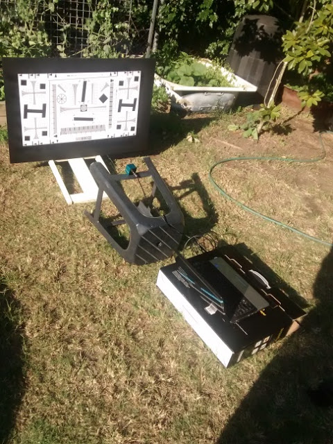
As you can see from my test apparatus below, this wasn't going to be a very scientific test.  The test pattern isn't completely perpendicular to the camera, but by doing the test outside I got as much light as possible on the board to take a good image.  For my analysis I'm only testing the vertical resolution just to double check the claims the manufacturer made.

Calibration Setup
Test Set-up
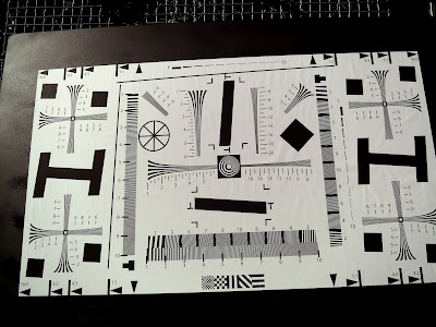
First up is the 8 MP ELP camera with a 3264 x 2448 sized image.

Test Pattern
ELP Camera Test Image
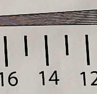
The lines on the vertical resolution test marker start to merge at about the 1400 lines per picture height mark.  As the picture in the image is 1750 pixels high, this mean that the image is a total of  1400*(2448/1750) = 1958 lines high.  This may seem small but it's 80 percent of the stated vertical resolution, and when you consider the non ideal test arrangement, and my eyeballing of the resolution chart, I'm satisfied that the resolution claims are correct.

Test Pattern
ELP Camera Resolution Limit
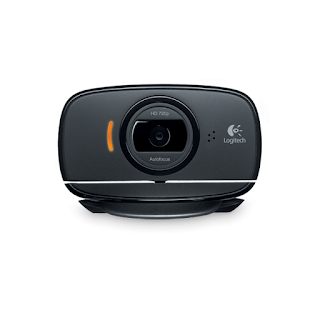
While I was at it I thought I'd test some other web cams.  First up is the Logitech C525 Auto focus camera.
WebCam
Logitech C525 Web Cam
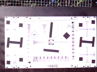
The test shot is at its maximum resolution of 1392 x 768.

Test Pattern
Logitech C525 Camera Test Image
In this case the markers merge at the 650 lines per picture mark.  As the picture is 600 pixels high this means that there should be 650 * (768/600) = 832 lines in the image.  Once again this is 8 percent higher than the stated resolution and when you take into account the errors in the measurement method, I'm happy that the stated resolution is correct.

Test Pattern
Logitech C525 Camera Resolution Limit
Finally, let's test my old C120 camera.

WebCam
Logitech C120 Web Cam
It produces and image with a resolution of 640 x 480.

Test Pattern
Logitech C120 Test Image
You're going to have to take my word for it, but the test markers merge at about the 350 vertical lines per image mark.  As the picture is 347 pixels high, the total image has a resolution of 350*(480/347) = 484 lines, which agrees with the specified resolution.

Test Pattern
Logitech C120 Camera Resolution Limit
In the end I'm verry happy with the camera it a good resolution and image quality for the price.

USB Cable Resistance

$
0
0
Just a quick post today.  I've been having trouble getting a Raspberry Pi with an attached webcam to take still images reliably.  I think it's a driver issue, but to make sure it wasn't a power problem I decided to sacrifice one of the cables that powers the Pi to make sure it was up to the job.  My concern was that the cable inside was so small it had a high resistance and when the current required for my application passed through, it would cause a voltage drop, resetting the Pi or causing it to lock up.  The cable tested was a 15cm cheap USB to micro USB cable with a braided fabric cover.

USB Cable
Micro USB cable
I initially did a quick measurement of the shield resistance.  Turns out the shields on both ends weren't connected to anything.  Not a good start.  The woven cover was then removed to reveal a plastic cable that contained 4 cores.  The ends of one of these cores was removed to allow its resistance to be measured.

USB Cable
USB cable core
I don't have a multimeter for measuring resistance values this low (accurately), so I ran 500 mA from a power supply through a single core and measured a 38mV voltage drop across the wire equating to a resistance of 76 mOhm.  That's not too bad.  I'm not considering the effects of contact resistance this is just to get a ball park figure to see if this cable is the source of my problem, and from what I can see here it most likely isn't.  The load draws about 600mA continuously which wouldn't cause a large enough voltage drop to cause the problems I'm seeing.  There's the chance that switching currents I'm not measuring are causing large drops, but I think it's unlikely.  To be sure, I tested a different high quality cable to power the Pi and got the same problems.

USB plug
USB plug solder connections

It thought the way the cable was constructed was unusual.  I'd expected some sort of crimp attachment, but I don't manufacture cables for a living, so maybe solder is the way to go.

USB cable
Wires inside USB cable

Looking inot the section of cable that I cut you can see that the middle two wires are closer together.  I assume this is because they are the differential pair of the USB cable and have a defined characteristic impedance.  In all, these cables aren't too bad.  They're fine for charging devices and supplying power to medium current draw devices.  As a side note I changed the webcam attached to my Pi and the problems seem to have gone away, which is a shame I really wanted to use the original camera.

RF LED Dimmer Teardown

$
0
0
I was recently contacted by someone that had read my post about MeanWell LED driver units with dimming capabilities.  They needed advice on how to connect a driver unit to a wireless dimming controller they'd purchased.  After a couple of attempts at connecting the two it became clear there wasn't a simple way to it because of the way they're designed.  After buying one for myself for 20 bucks I thought I'd do a teardown and analysis of how the wireless dimming controller works and explain why they can't easily be connected.

RF LED Dimmer
The wireless dimming control unit is designed to operate from a 12 - 24 volt input and vary the brightness of a regulated load up to 8 Amps via PWM switching, whereas the MeanWell LDH-45 driver is a DC-DC converter that has an input terminal to switch an unregulated load on and off in a PWM manner.  The PWM input has a maximum input voltage of 8 volts, I think it can do more but the documentation is unclear.  So in theory we can put a resistor divider across the 12 V output of the dimming controller to reduce the voltage to a safe level and connect it to the PWM control terminal.  See if you can spot the mistake I've made in my logic.  I'll explain it later on but needless to say the connections in the diagram below wont work.  I'll give you some clues disconnecting the positive output of the dimmer causes the light to go out, but disconnecting the PWM DIM terminal causes the light to stay on.

Initial Incorrect Connection


A 3 button remote control key fob unit is used to increase and decrease the brightness of the lights as well as turning them off.

Remote control key fob
For the low price I paid I expected the remote to be a low quality PCB with cheap components in a flimsy case.  Surprisingly the remote control is well built, with a water resistant rubber seal.

Rubber waterproof seal
There isn't anything too interesting in the remote.  It contains a user replaceable battery, some surface mount tactile buttons, and a status LED.  The marking on the crystal indicates that unit operates at 433.92 MHz.

Remote control PCB
The main dimming unit is also reasonably well constructed for such a cheap item.  Although screw terminals would've been nicer, it comes with spring loaded connectors like you'd see on the back of a set of speakers.  These are directly soldered to a medium quality single sided board of low complexity.

Bottom of LED Dimmer PCB
After the board is removed the operation of the device becomes clearer.  You can see that it contains a radio module (with a coil of wire for an antenna) that communicates with the key fob, some memory, an unknown microcontroller, a switching FET, a pull up resistor for the I2C line, and 3 extra components that make up the power supply.  The board is name "RF-DIMMER-MBK-V7"

Top of LED Dimmer PCB
The memory IC is an ATMEL 24C02N 256 byte serial EEPROM device.  I assume this is used to store the  device state as it returns to its previous on/off and dimming state if power is removed and reapplied later.

ATMEL 24C02N - 2048 bit serial EEPROM
The RF control module is connected to the board via a 4 pin header.  Two of these are connected together and I assume send data to the microcontroller.  The other two are 5 volt and ground lines.

RF Module PCB
Although it's incredibly hard to see, the switching MOSFET is a 50N03-10 CP device.  It has a 30 volt maximum VDS and a maximum drain current of about 50 Amps (Not at the same time of course).

Switching MOSFET
To explain why the device didn't operate as I first expected, it helps to colour code the different nodes on the circuit board below.  Once again the input is on the right.

Black - The negative input terminal and ground point for the rest of the circuit.
Red - The positive input terminal.  It's directly connected to the output positive terminal and supplies power to the rest of the control circuit.
Purple - This is the input voltage after is has passed through a reverse protection diode
Yellow - This is a 5 V line supplied by 7805 voltage regulator
Dark Blue - This is the data line that is returning from the RF module
Light Blue - The Mosfet gate drive
Green & White - SDA and SCL lines of the I2C bus
Orange - Negative output terminal

Voltage Node on PCB
To help make it even clearer why my first connection attempts didn't work I redrew the schematic in a more conventional fashion.

RF LED Dimmer Schematic
As you can now see, the circuit is relatively simple. It takes the input voltage through a reverse polarity protection diode and feeds it into a linear regulator to provide a 5 Volt line.  This is used to power the memory IC, RF module, and unknown microcontroller.  The microcontroller reads data from the RF module and stores this configuration data in the EEPROM memory.  The microcontroller then adjusts the PWM waveform driving the gate of the MOSFET turning the load on and off rapidly and changing the brightness of the light.  It does this by effectively disconnecting the negative terminal of the load.

Why my first idea didn't work is becoming clear.  I assumed that the switching element would be on the high side of the load with the load connected to ground and the switch between the load and the 12 volt line as in figure b below.  Connecting a voltage divider as a load would have produced a PWM signal between 0 and 6 volts, but this wasn't the case.

The switching mosfet is on the low side of the load as in figure a below, and for a good reason too.  This allows the gate drive voltage of the mosfet to be independent of the supply voltage.  A high side switch would require a p-channel mosfet and a gate voltage of 5 volts less than the input to drive it, but because the input voltage can vary from 12 to 24 volts the gate drive voltage would also have to vary.  This can be done, but it adds extra parts.  It's much easier to use a low side switch and drive it with a 5 volt signal that doesn't change as the input voltage does.  Placing a resistor divider across an output like this will give a PWM signal that changes between 6 and 12 volts.  This means that the light will come on and stay on.  Disconnecting the positive output of the dimming unit will cause the PWM DIM and the -DIM terminals to be connected with a resistor, placing 0 volts on the PWM DIM turning the light off.  If you disconnect the PWM DIM line the light will turn on as mentioned in its data sheet (leave unused wires unconnected).

The MeanWell LED driver really requires an output configuration similar to figure c, where the output terminal is forced to high or low voltage, the other configurations can force the output to a high or low voltage but not both.
Load switching configurations. Assume 12 volt input on the left of each figure, load on the right.
To look at the waveforms of the dimming device.  I placed a dummy load resistor on the output and measured the voltage across it.  The image below shows the device at two of its 32 dimming settings.

Voltage across load at dimmest setting
Voltage across load at approximately quarter-brightness
After thinking about it, there is a way to connect the unit to the MeanWell controller.  The voltage used to drive the FET is exactly what we need to drive the PWM DIM pin.  So if you were to open the box and solder on a wire to the light blue trace in the above diagram everything should work.  Bringing the output of a microcontroller out to the real world without protection isn't ideal, and the current the microcontroller can supply is unknown.  You could give it a go, it should work.

Voltage on the MOSFET gate
As an aside my initial tests were with a long strand of LEDs and I got some strange results.  What was happening here was when the low side switch was turned off the cabling in my setup was coupling in noise from the mains voltage.  Testing with a resistor fixed that though.  Doh! 
Initial incorrect experiment

LED Array Test PCB

$
0
0
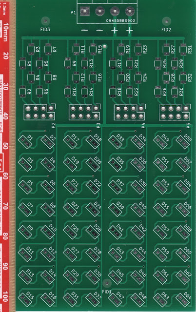
A quick post today.  I was discussing the idea of an illuminated display recently and was unsure of how bright LEDs would appear when driven with different currents.  After looking around, I found some nice 100mA white LED devices and thought I'd make a PCB to do some tests. My original plan was to make a 7x7 grid of 4 LED clusters for a total of 196 lights, but the price of the PCB was too much.  As I'm using a prototyping service that gives me 5 copies of the board I decided to break it up into smaller boards that could be tiled.

As this was for testing, I wanted the lights to be configurable, so each cluster of 4 LED's goes to a standard pin header.  To power a cluster, you just add a jumper to the header.  Simple.  The board also includes some current limiting resistors to help current sharing, but the board isn't designed to be a standalone device, and needs external control to be driven properly.  This is why the header pins are in between the LEDs and the resistors.  If needed an external connector and be plugged onto the header pins to drive the LEDs, removing the resistors from the circuit.

After weighing up my objectives I decided to use 20 ohm resistors to limit the current, but at 100 mA the dissipated power would be 0.2 Watt.  It turned out to be more economical and flexible to use 2 x 10 ohm resistors instead of 1 x 20 ohm.

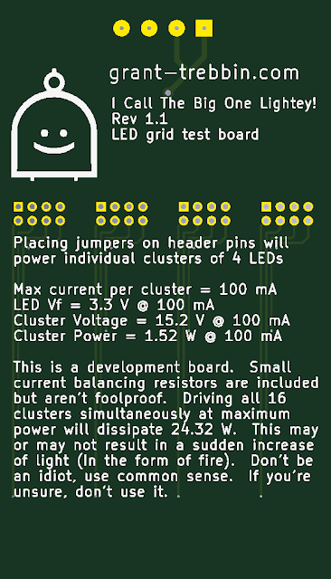
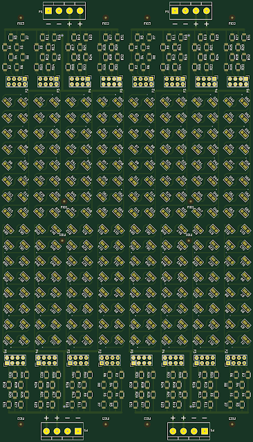
PCB Rendering
Top Layer
Breaking the board up into smaller portions is probably a blessing.  I'm not even sure I can solder these let alone a board that had something like 300 components, but I'll give it a shot.

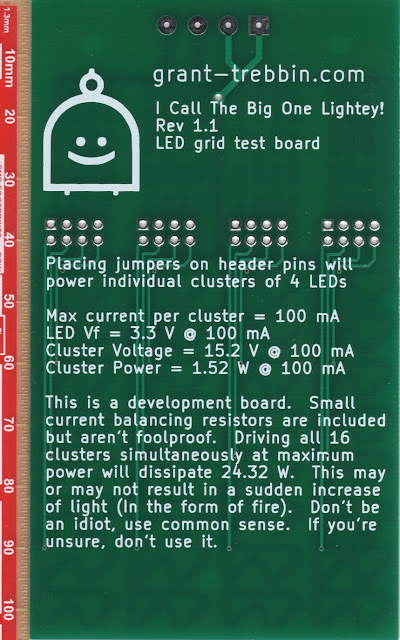
When designing boards, if possible, write some notes on them so you'll know how to use them in the future.

PCB Rendering
Bottom Layer
I'll release the boards after a little more work (pressed for time at the moment)

PCB Rendering
Tiled PCBs

A Basic Discrete Event Simulation

$
0
0
Let me paint a picture.  You run a service station (or gas station for our American friends), and you sell bread.  It's a 24 hour business with a uniform flow of customers throughout the week and you want to investigate the effectiveness of the ordering routines you use.  How do you do it?  The answer is Discrete Event Simulation.

I'm ashamed to say I've never heard of it, and once again came up with the idea independently  (Another case of "Wouldn't it be cool if ........  *Googles*  Oh, this already exists, is well developed, and people make a living from it").  I'm familiar with the simulations used in designing electronics, but had never experienced this type.  Basically a queue of events with timestamps is created, the next event is removed and processed and this is repeated until a certain time or all the events have been processed.

The reason I'm looking into this is because I have something I want to simulate and had originally planned to use the Simpy simulation package for python, but as I started working it became apparent that it was overkill for what I needed.  It's great for simulating resources that interact with each other, and although it looked like my problem needed this it really didn't.  The ordering process and customer process don't interact, even though it looks like they do.  I'm referring to the time that events occur.  Customers arrive indepenently of each other and of when deliveries happen.  They are linked by the stock levels in the store but this is handled by a stock on hand variable (My basic scenario above could probably be handled by Simpy, but I plan for it to get complicated).

After much procrastination I decided to write my own, but as it turns out someone has done the hard work for me.

User GaretJax  from http://codereview.stackexchange.com/questions/3670/discrete-event-simulation-with-variable-intervals already had a basic framework for this problem.  So I ran with it.  (Check github for  DiscreteEventSimulator.py)

The first thing to do is describe the processes at play.  The customer for example is described below.  They walk in and if bread is on the shelves, they buy a loaf and the stock on hand is decremented.  The time until the next customer is described by an exponential distribution to simulate a poisson process.  The final thing to do is schedule the next customer arrival.  The sales rate is 0.0004 loaves per second, or more intuitively, one loaf every 2500 seconds or around 40 minutes.

Python Code
Customer Process

The ordering process is very simple.  The bread delivery truck turns up and the staff member counts the stock the store currently has, and then works out how many loaves are needed to bring the stock levels back to 50 loaves.  But there is a small problem.  Loaves of bread only come in crates of 24.  So they need to round up to the nearest multiple of 24 and take that from the driver.  This is then added to the stock on hand.

Python Code
Order Process

All that's needed now is to start the simulation.  7 events are created for the bread deliveries, one for each day of the week at 1 am.  An initial customer is also scheduled.  Only one is needed as each customer generates the next customer event.  I've then set the simulation to run for a week.

Python Code
Simulation configuration

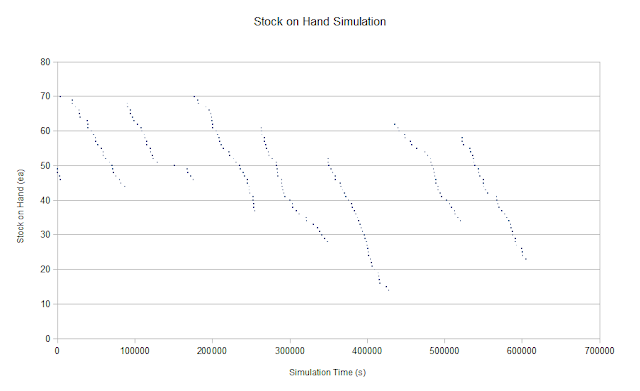
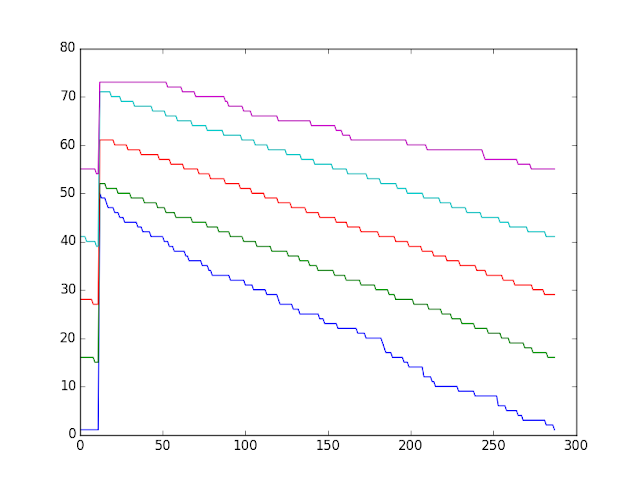
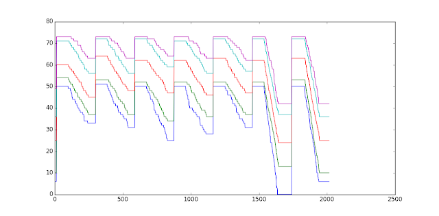
The results below starting from Monday are interesting.  We can see the random nature of the purchases, but the overall trends are visible.  We can see that on Monday, Tuesday, Wednesday, Thursday, Friday, and Sunday, only one crate a day was needed, but on Saturday two crates were needed.  It's also possible that they're holding too much stock as for the first 3 days of the week the stock barely falls below 40 loaves.  (Customers have been complaining about stale bread, maybe this is the reason.)

Stock Graph
Simulation Results
This is only a quick overview of the process with some very simplistic assumptions and modelling, but I've got a framework to use now and I have thoughts on how to make this more realistic (and complicated).  This problem has been kicking my arse all week,  I only managed to pull it all together in the last couple of hours.  Very happy at the moment


https://github.com/GrantTrebbin/DiscreteEventSimulator
Get the code!


Breadboard Killer Review

$
0
0
I recently did a post about a small PCB to test out some surface mount LEDs.  Apart from the main objective of seeing how bright LEDs appears under certain lighting conditions, there were several other reasons for designing the board.  I hadn't designed a PCB in a long time and had an itch to make one, there was also curiosity about how Kicad had progressed since I'd last used it.  For this board I'm also going to use a stencil for the solder paste for the first time.  It never hurts to learn new skills.

The other reason I wanted to do this was to test out a small volume PCB prototyping service called Breadboard Killer.  It's an Australian company and I really like the name.  The use of breadboards has basically become unsustainable.  It seems ridiculous that I still see them in use at universities.  If you're training people to design contemporary electronics that run at high frequencies and use surface mount components, starting with breadboards is a set back.  Sure, give them a one to wire up a 555 timer with a blinking LED to get them started, then throw an EDA tool at them.  If you know your stuff, and have faith that the schematic you design works, just go straight to PCB.  They're are cheap, and if you screw up, who cares.  That's why PCBs have Revision numbers and Kynar wire was invented.

So how did the boards turn out?  Really well.  For $56 Australian I got 5 copies of a board that's 10.5cm x 6cm.  The boards have nice clean routed edges and don't have rough bits where break away tabs are left behind.  The board house does add a serial number, (seen in the footprint for the terminal connector in the image below) but that's standard.

PCB
Top Side of PCB
The silkscreen is high quality and very sharp, whereas the silkscreen on some other boards I've seen for other manufacturers look pixelated and blocky.

PCB
Bottom Side of PCB
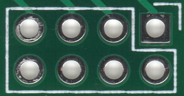
The image below shows the registration between layers.  The drill holes seem to line up well with the copper layer, but there is a small offset in the solder mask.  That's nothing to worry about and is completely within specification.  That's why you have solder mask expansion after all.


PCB
Header Footprint
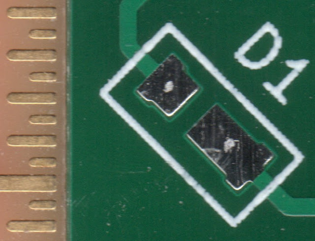
It's hard to see in the image below but the footprint of the LED I'm using has pads that are slightly T-shaped.  The right angles in the corners are slightly tapered, but that's to be expected.

PCB
LED Footprint

The ordering process is easy too.  I had a slight problem with the files names I used, but that was quickly resolved.  The site also generates a nice render of the uploaded gerber files as a final verification step to make sure that all the layers are correctly identified.  I intended to make my project open source and share it on the site, but I think I needed to include a license in the zip file I uploaded and I didn't realise this until I was part way through the order process.  I'll look into that for next time.

UPDATE:  Matt from Breadboard Killer let me know that you can make designs open source after submitting the project by going into your account and editing the project.  So I've gone ahead and done that.  Here is my project page https://breadboardkiller.com.au/designs/55-ledgrid.

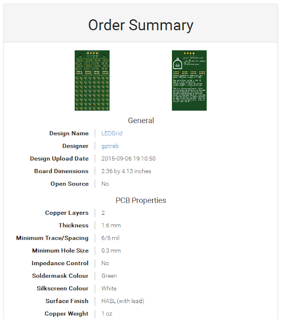
Order Screen
Order Confirmation

The order took 19 days to arrive.  I picked the cheap slower option that has a range of 8 to 20 days, so everything is OK there.  The price is pretty reasonable as well.  It's hard to compare this to services like OSH Park as they have different capabilities and multiples of boards.   I'll have a go though.

As of 27 - September - 2015

Breadboard Killer - 5 boards shipped for 56.18 AUD
OSH Park - 3 boards shipped for 48.82 USD ≈ 69.50 AUD

To be fair the OSH park boards have an ENIG coating on the pads, but most of the other specs are the same.  OSH park could also look expensive due to recent changes in the Australian dollar.  Not sure, but I think the breadboard killer PCBs are made in Singapore.  This is based on the Singapore Post shipping option.

All up I'm really happy with the quality and services Breadboard killer provides.  I've recommended them to a couple of people and I'll use them again.  Now I just need to wait for my solder paste stencil before I can have fun.  :-)

Generating 2 Level Harmonic Elimination PWM with Python

$
0
0
A couple years ago I wrote some code to generate Harmonic Elimination PWM (HEPWM) waveforms in octave, which is kind of like Matlab.  Recently someone asked if I could rewrite it in Python so it'd be easier to use and understand (fair call, it was pretty archaic).  I jumped at the chance as I'd been meaning to do it but just didn't have a strong reason to.  While I was at it I added a feature that may make it more useful, but more on that later.  To understand everything I recommend reading my previous HEPWM posts.

I should take a step back and first explain what HEPWM waveforms are.  If you're reading this I'm going to assume that you know what a PWM wave is and that you know the square nature of periodic PWM waves generate unwanted harmonics.  HEPWM is an extension of that idea, but the timing of the transitions in the wave are calculated to cancel or reduce specified harmonics.  The even harmonics are eliminated by default by making the wave half wave symmetric.  You don't have to make the wave quarter wave symmetric, that's a bit of a maths trick, but by doing that you halve the number of equations and unknowns that you need to solve for.  (If I remember correctly, solving the entire set of equations allows you to control the phase of the harmonics as well.)  That sounds really complicated, but the image below may help.

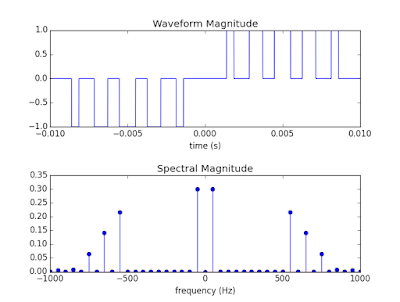
The upper waveform is typical of what you'd see on the output of an unfiltered inverter.  In this case the period of the wave is 20 ms, which means the fundamental frequency is 50 Hz.  The HEPWM calculations however have allowed the creation of a wave with the 3rd, 5th, 7th, and 9th harmonics set to zero and the fundamental frequency set to 0.6 (It looks like 0.3, but you have to remember that the positive and negative frequencies add in this case)  As we're controlling 5 harmonics (1, 3, 5, 7, 9) there needs to be 5 transitions in each quarter of the waveform.

Waveform
3 Level HE-PWM
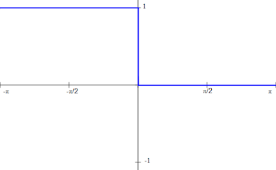
The HEPWM waveform is constructed by starting with the base waveform below.  Multiple versions of this waveform are alternatively added and subtracted with the alpha values increasing each time (Alpha values are always between 0 and T/4)

Waveform
Quarter Wave Symmetric Waveform
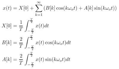
Start with the definition for the Fourier series below.  It can then be applied to the above waveform.

Equation
Fourier Series
If you do the math X[0] = 0, B[k]=0 and A[k]=0 for even positive values of k.  For positive odd values of k, A[k] is shown below.

Equation
Fourier Series Coefficient for QWS waveform
This is the magnitude of a particular harmonic, k, for a particular value of alpha.  The total value for each harmonic can be found by adding all the components from each value of alpha (remember alternating alpha values cause the sign to change).  It helps to note the relation between the period and angular frequency.  Combining this with the above equation a system of equations can be generated and solved.  I go into more detail in previous posts, but this is needed to give context to the next addition.

Equation
Angular Frequency
The 3 level waveform in the first image is easy to generate with a H bridge topology, but what if you want to accomplish a similar effect with a microcontroller with only 2 output levels?  It seems that you can just shift the first half of the waveform up by adding the waveform below, but by doing that you are adding the Fourier series of the below wave to the Fourier series of the waveform calculated above.  This will invalidate the magnitudes of the harmonics you are trying to target.  I reused some images from a previous post that used a period of T but it makes more sense to use a generalised period of 2 pi.

Waveform
Translated Square Wave
All is not lost though, calculating the Fourier series of translated square wave above gives the result below.  There's nothing we can do about the DC offset, but the summation term can be easily added to the  calculated harmonics of the original waveform because it only has a sine term.  All we need to do is tweak the code the generates the set of simultaneous equations to be solved and we can now move to a 2 level system.

Equation
Fourier series of Translated Square Wave
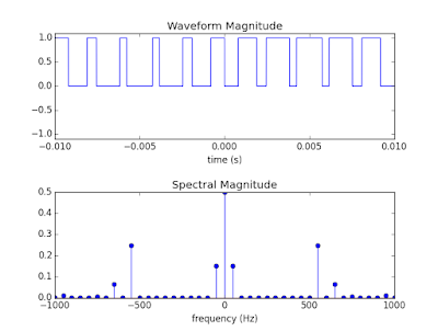
 For clarity, a two level system with the 3rd, 5th, 7th, and 9th harmonics nulled and the main harmonic set to 0.3 is shown.  The main difference between the spectrum of this waveform and the one above is the DC offset.  That's what coupling capacitors are for.

Waveform
2 Level HEPWM
Below is the python code that does this little trick.  When the twoLevels variable is set to 0, the code runs as usual and generates the transition points for a 3 level waveform.  When it's set to 1, the adjustment term that describes the Fourier series of the square wave is included in the calculations.  (What the hell was I thinking with that comment "the location of the switching location")

Python Code
Calculating the Harmonic Magnitude in Python

Caveats, Warnings and Errata

This code isn't meant to hold your hand.  It's a demonstration and will probably have errors.  If you find any let me know.  It also assumes that your waveforms have perfect 0 time transitions with no overshoot or similar real world effects.  I recommend using it as a starting point.  Calculate your transition points and do a localised search with those values while running simulations closer to the real world.

I did my best to document things, but it's hard to comment symbolic math equations.  I may look into that.

Get the code!


Process an MBOX file with python

$
0
0
Getting snowed under with email?  Before you go and clear it all out, have a read of this because it may prevent the same thing happening in the future.

I'm on holidays, and one of the first things on my to do list was to clean out my inbox.  From what I've heard of other peoples experiences, my 400 email inbox isn't too bad, but it was getting unmanageable.  It's been that way for a while and I eventually got to a point where I didn't delete anything and just let it build up.  I did that for a reason, I wanted to analyse all of the email to see where it was coming from.  That way I could take appropriate action to change email settings on services, unsubscribe from things, or set up some filters.  By investing some time now, I can reduce my ongoing maintenance.

I wasn't sure how I was going to go about this.  I originally thought that I'd have to use something like a google apps script to retrieve data from my email account, but as it turns out Google finally got their act together and now have a way to download an archive of your email.  They even give you the option to select specific labels to include in the downloadable MBOX file.  This is handy as I only want the emails in the inbox.

download settings
Email download process


From this point things were easy.  Python is able to parse the MBOX file and extract the required information from the emails.  The subject and sender emails addresses were extracted and processed with the following procedure.

1.  Split the strings at whitespace
2.  Remove everything except alphanumeric characters
3.  Convert the string to lowercase

All the results were combined and then sorted and counted to give a result similar to the below image.

word frequency
Email word frequency

It's not perfect, but it gives you a quick way to identify problem areas.  Watch out for Unicode problems though, I think I've taken care of it but it's hard to tell.

Github Gist

Using a Solder Paste Stencil for a Prototype

$
0
0
If you've seen any of my previous post you'll know I'm in the process of making a PCB that contains a configurable LED Grid.  Why?  Something to do I guess.  Anyway I finally got around to assembling the board I had made by BreadboardKiller.  I've assembled small surface mount PCBs in the past and have always manually applied the solder paste by hand with a syringe.  It's hard to get right, you might not get paste in the right place, you can use to much or too little, but when it's a only a few parts it's not too hard to fix.  This board has 96 surface mount components on it, which means that doing it by hand was going to be a close to impossible.

I decided to get a laser cut Kapton stencil from OSH Stencils.  At 40 dollars it looks expensive for a piece of plastic, but that includes a one off cost for set of board holders the exchange rate wasn't kind either.  These are the black acrylic L shaped pieces in the image below.  The stencil was only 20 dollars US which was well worth it.

There are demonstrations on how to use the stencils online but I'll show my setup.  The board holders are taped down and the stencil is aligned and taped down on on side to act as a hinge.  This allows a board to be put in the holder, have the stencil flipped over it, the paste applied, the board removed, and the process repeated.  Application of the paste is easy.  Squirt some out of the syringe where it needs to go, and use the paste spreader (basically a credit card) to swipe the paste across the stencil.

PCB Assembly
PCB Assembly Set-Up
The stencils are easy to use and make sure you apply the right amount to each pad.  For this project I chose to use lead free solder as I assumed that I'd get it everywhere when using the stencils.  I was right.  I wasn't sure how to clean it but mild soapy water did the job.

Solder Paste Stencil

Solder Paste Stencil
Part of Stencil for LEDs

Solder Paste Stencil
Part of Stencil for Resistors

Solder Paste Stencil
Stencil label
Once again I used my toaster oven to solder the boards.  It has no automatic controls, I stand there and watch the board and time the steps by counting aloud to myself.  The temperature is also set manually by turning the dial.  The process is described in a previous blog post.  It helps to put a little bit of solder paste on a fiducial mark so that I can see the moment the solder liquefies through the oven window.

PCB Reflow
PCB in Oven After Reflow
It's important to shield the board from direct IR radiation from the heating elements, that's why there are trays above and below the board.

PCB Reflow
PCB in Oven after Reflow
After the surface mount parts were soldered the through hole parts were added by hand.

PCB
Assembled Board with LEDs
When I designed the board I screwed up and made the holes in the footprint for the terminal blocks too small.  This means they had to be enlarged by hand, and because of the way the tracks were laid out, the positive terminal block has to go on the other side of the board.  No biggie.

PCB
Assembled Board

PCB
Assembled Board

Surface Mount Resistors
The parts seem to have been soldered nicely.  There isn't an excess of solder or too little, and there's that nice little fillet you expect to see as well.

Surface Mount Resistors
0.25 Watt 1206 Resistor
The LEDs are harder to judge as the pads are under the board, but they all work.

Surface Mount LED
Osram GW JCLMS1.EC-GUHQ-5L7N-1 LED
Just to prove they all work.

LED Grid
LED Grid
To show the reconfigurable nature of the board I disconnected the jumpers that power the middle section of the LED grid.

LED Grid
LED Grid with Sections Turned Off
Over all I'm very happy with the results.  Obviously boards produced this way aren't going to be of the same standard as professionally made ones, but these are rather sturdy and fine for prototypes.  I'd gladly use OSHstencils again just for the time that it saves me.

Monte Carlo Simulation and Discrete Event Simulation

$
0
0
I've been doing some more work on my discrete event simulator, or to be more accurate, the supporting functions that help to analyse the results.  In my previous post I described a basic stock management situation that can be modelled.  I'll continue to use that model here as it's simple to understand and helps illustrate the features I've added.

To bring you up to speed, the simulation models a 24 hour, 7 day a week business that gets deliveries at 1 am and sells items all day.  It's not realistic but it's a starting point.  The main problem with it is the discrete random nature of the events.  This can be seen in the week long simulation below from the last post.  It's possible to identify trends and events, but it offers no insight into how likely these events are to occur.

Simulation Graph
Original One Week Simulation

Getting data about the likelihood of events occurring can be accomplished by running the simulation for a longer time period and then comparing smaller sections of the simulation.  In my case I ran the simulation for 200 weeks, broke the data up into weeks, and then performed analysis on those multiple trials, just like a Monte Carlo simulation.  These results can be seen below.

The graph illustrates the exact same model, but instead of one trial, the model is essentially run 200 times.  This allows percentiles for the simulation to be generated.  In this case 0, 10, 50, 90, 100.  To put this into more understandable terms, in the graph below, 0% of the simulations predicted stock levels less than the dark blue line, 10% predicted levels less than the green line, 50% predicted levels less than the red line, 90% predicted levels less than the light blue line, and 100% of the simulations predict levels less than the purple line.

Simulation Graph
A monte carlo analysis of a discrete event simulation
This kind of analysis allows sensible measured conversations about stock levels to take place.  All to often predictions are made that don't allow nuance and can cause problems.  For example, instead of saying "I reckon we'll run out of stock by 1pm"  we can now say "There's a 40% chance we'll run out by 1 pm".  Everyone can take that on board and take appropriate action, it may be a 40% chance is acceptable as there may be some other more urgent matter to take care of.

I'm anthropomorphising the conversation, but in reality I see this as a way for computers to compare and prioritise tasks.

You may have noticed a problem with what I've described.  The original data from the discrete event simulator isn't a regularly sampled data set.  A customer may come in 10 minutes after the last one and then you won't see another for an hour.  To perform the Monte Carlo simulation the data needs to be resampled with a regular timebase.  In my case I've choose to sample the data every 5 minutes.

This is done with a kind of zero order hold.  The process to determine the value at a specific time is straight forward, if an event occurs at this time the new data point will be the value after the event.  If there is no event, the data point will be the value after the last event.  If there is no previous event the first one is used.

The image below illustrates the initial data set of (1, 1), (5, 2), (10, 3), (11, 4), (12, 5), (20 , 6).  These are marked with blue crosses.  The red line shows how this data is resampled for different points.  The black bars show the result of resampling the data at -10, 1, 2, 10 and 30.  The results are 1, 1, 1, 3, and 6 respectively.  I've chosen to resample the data at 5 random points, but if performed at regular intervals the information is ready to be fed to the Monte Carlo analyser.
Simulation Graph
Resampling a data set
To give a usage example I've folded the entire simulation into a period of one day.  That means there are 1400 days sampled every 5 minutes simulated and compared in the image below.  If I had concerns about the stock levels at 8:50 pm (sample 250), I could look at this and say that I'm very confident that there will be stock, if fact there should be about 30 to 50 items available.

Simulation Graph
The simulation folded into a single day
In the simulation below I've increased the sales rate so a different question can be asked.  If customers complain about out of stocks you can look at this and say that supplies will run out somewhere between 7:30 am and 3:50 pm (90 and 190), but most likely at 10:50 am (130).  This then allows you to take action, such as increasing the order size.

Simulation Graph
Increase rate of purchase indicates likely stock exhaustion points
It's all a bit simplistic at the moment, but it's getting there.  What I'm really aiming to show is the complex interaction of seemingly unrelated variables.
https://github.com/GrantTrebbin/DiscreteEventSimulator
Get the code
.

Adding a Sales Profile to a Discrete Event Simulation

$
0
0
If you've been following along, you'll know I've been putting together a discrete event simulator for inventory management.  The goal is to better integrate knowledge of sales history, stock levels, and ordering patterns to make quantitative decisions about what to order and when.  So far I've been using a scenario involving a 24 hour business with a constant sales rate, but that's not realistic.  Therefore the next step is to add a way to generate a customer flow based on a sales profile.

The way I've gone about doing this is to start with a graph of a sales profile.  Let's slightly change the scenario I've been using.  We're now looking at a profile of sales at a fruit shop.  The fruit shop only opens between 8am and 9pm on weekdays, 8am to 5pm on Saturdays, and 9am to 6pm on Sunday. Weekday sales are $3000 a day, and weekend sales are $7500 a day.  This is a total of $30000 per week.  When graphed against seconds passed, the total sales for the week are shown below.
sales graph
sales profile
In the previous simulations I was modelling the customer flow as a poisson process, where item sales per second was used to generate random times between customer arrivals.  This makes it hard to create a varying sales pattern based on customer flow.  This is easily changed though, you just need to interpret the problem differently.  If for example 150 watermelons are sold per week, that means that on average $200 are spent in the store as a whole between each watermelon purchase.  If we assume that the customer flow of people buying watermelons is similar to those buying fruit in general, which in the absence of better data is a reasonable assumption, a sales pattern can now be generated.

If instead of saying "a customer will buy a watermelon at x seconds into the week" we now say "a customer will buy a watermelon at x dollars into the week", it makes sense to reverse the situation and use the sales as our independent variable.  The way to do that is indicated in the image above.  The evenly spaced horizontal black lines indicate sales increments of $1000.  When projected across to the sales profile and then down to the time axis, a customer flow is generated.  You can see that there won't be any sales when the store is closed as the line can't intersect with these time periods.  Days like Saturday and Sunday that have a high rate of sales intersect a lot of lines and project them into a small time period.

I've written a custom class to perform this interpolation process on a piecewise function that's passed to it.  It allows a dollar value to be converted to a time stamp and vice versa.  The supplied interp function in numpy is almost adequate, but it has some extra constraints placed on it.  Firstly the data supplied needs to have unique timestamps in increasing order, it doesn't make sense to have two different sales values for a single point in time.  The other requirement is that the sales data needs to be increasing, in this case it's fine to have two data points the same, it just means no sales have occurred in this period.

To ensure consistency, I wanted to ensure that when converting from dollars to time, predictable and consistent results were produced.  This may not seem obvious, but if you were to convert the dollar value of 3000 to a timestamp in the above example there are multiple answers.  Any time between closing on the first day and opening on the second day the sales value is $3000.  I decided to make it so the earliest time a particular dollar value is reached would be returned.

It's simply a matter of creating a piecewise function as shown below.  It can be as detailed as you want.  I've only indicated sales at opening and closing times and linearly interpolated between the data points, but you could supply hourly or minute by minute sales data if you wanted.

python code
specification of a sales profile

Using this function, a customer pattern is generated in terms of dollars and then back projected to timestamps.  These values are then used in the simulation.  I haven't changed the ordering requirements from the previous scenario.  You have to order 24 items at a time, the deliveries happen at 1 am, and after the delivery driver has left, you have to have 50 or more items.  So what does the simulation look like now?
simulation results
stock on hand simulation with sales profile
You can see the plateaus where there are no sales because the store is closed.  The deliveries at 1 am also appear as interruptions to the plateaus.  Also visible are the slow weekdays sales of $3000 over 13 hours.  This can be compared to the weekend sales of $7500 over 9 hours.  This increased rate of sales of approximately 3.6x on a weekend is visible as well.

I'm not happy with my code at the moment so I'll take some time to refactor it and change some of the terminology to generalise some parts.  My main concern at the moment is to create good libraries, the test.py program is sort of a test bed for these.
https://github.com/GrantTrebbin/DiscreteEventSimulator/commit/eb24b7c44298c428170db3490f4d57e4062de7af
Get the code!

Viewing all 99 articles
Browse latest View live